Dice (Part 2 of 2): Context Free Grammars, Random Walks and Fractals

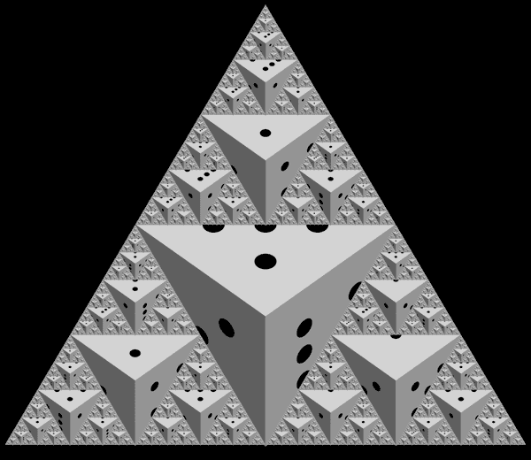
In Part 1, we took a look at the various mechanisms and theory driving probability distributions on dice. Now, equipped with some new distributions using edges and corners of the die, let's find some applications for them. In this post, we'll show an algorithm for generating a random die corner (motivated by the group theory section of Part 1) and then use this distribution to visualize random walks and branching processes. These visualizations will turn our attention to the realm of fractals. I'd recommend reading the first post in order to fully appreciate this one.

Context Free Art

Context Free Art (CFA) is a programming language focused on the production of art from code. What makes it unique (from, say, processing or p5.js) is that the CFA language is designed as a context free grammar (CFG). CFGs are studied in the field of formal language theory — see the Wikepedia article for more information on them.

A CFG is a set of rules describing the production of valid words. For instance the following grammar produces strings like $ab$, $aaabbb$ or any string of the form $a^nb^n$.

This notation says that a valid word is produced by a single production rule $R$. $R$ is either (1) expanded as another $R$ sandwiched between $a$ and $b$ or (2) is an empty word ($\epsilon$ is used in formal languages to mean the string of zero length). This is a recursive rule, meaning we can apply R multiple times until we decide to terminate the word.

CFA programs look similar in essence to the above language, in the sense that programs are formatted as (usually recursive) production rules. In CFA, the rules are not thought of as producing words but more so as producing drawings. Let's look at an example program.

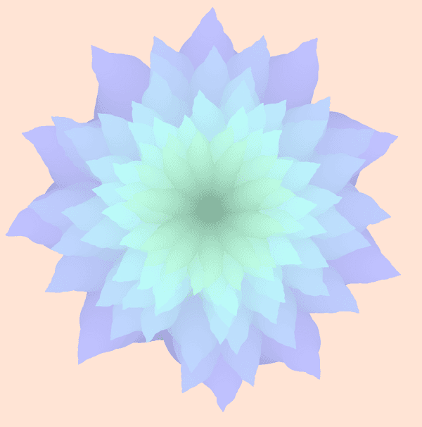
startshape FLOWER
CF::Background = [h 20 sat 0.2]

shape FLOWER
{
loop 10 [s 0.9 r (360 / 11 / 2) h -10]
  PETAL_LAYER [ h 240 sat 0.3 b -1]
}

shape PETAL_LAYER
{
  loop 10 [r (360 / 10)]
    PETAL [s 1]
}

shape PETAL
rule {
  CIRCLE []
  PETAL [s 0.995 b 0.01 x 0.01 y 0.005]
}
rule {
  CIRCLE []
  PETAL [s 0.995 b 0.01 x -0.01 y 0.005]
}

This program says: "Draw a flower. A flower is made up of 10 layers of petals. A layer of petals is 10 petals arranged in a circular pattern. A petal is a bunch of circles that shrink and wiggle a bit side to side." The drawing from the beginning of this section was produced by this program.

A fun graphic from such a short program!

Algorithm for a Random Die Corner

Let's use CFA to apply our new knowledge of dice distributions from Part 1. The goal will be to write a CFA program to generate and render a random die corner.

The first step, generating a random die corner, is an interesting coding problem. From Part 1, we know that there are 24 possible outcomes including the orientation of the die. How do we go about elegantly describing the production of a random corner? We'll work by choosing a starting position of the die and then applying certain rotations such that all 24 outcomes are equally possible.

Start with the corner $(1,2,3)$ (say that 1 is facing upwards). Then proceed as follows.

1. Randomly decide whether or not to rotate the cube upside down such that the 6 is facing up instead of the 1.
2. Randomly rotate the die by 0, 90, 180 or 270 degrees while keeping the top side facing up.
3. Randomly rotate the corner by 0, 120 or 240 degrees.

The axes of rotation are visualized in this animation.

The first step has 2 possible outcomes, the second has 4 and the last step has 3. Altogether, that's a potential $2 * 4 * 3 = 24$ outcomes. In addition, we're hitting each outcome exactly once (try to verify this!), meaning we have a correct algorithm by which to generate a random corner.

It's worth noting that the algorithm preserves the chirality of the die through the usage of rotations. Without the knowledge of chirality that we gained in Part 1, it's easy to make the mistake of writing an algorithm which accidentally produces die corners of differing handedness, which would not be possible with a physical die.

Rendering the Corner

CFA describes the production of two-dimensional drawings, but we want to render a three-dimensional die. In order to make this work, I had to apply some knowledge of linear algebra to construct a matrix transformation to give the visual effect of three dimensions. This includes the use of affine transformations, change of bases and projections in order to properly do so. I've decided to leave out the details here, but maybe I'll revisit the math of computer graphics in the future.

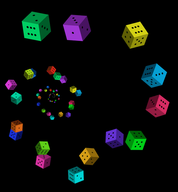
Now, using the die as a primitive object, we can apply it to generate fun drawings with recursive rules just as we did with the flower. Here's a neat one which renders dice falling in the shape of a spiral (with each die being a randomly generated corner). I call it "Out of Luck".

Random Walks

Let's go for another program that takes advantage of the outcome of the dice and visualizes it in some way. First, we'll simulate a random walk. What we'll do is: If the die roll is even, we'll move the die further away and if it's odd, we'll move it closer to the camera. Here's the result of one random output.

You can see the series of rolls of 1s in which the die moves closer before we see a 2 after which it starts moving away. Again, this a random process. So we could run the program again and get a new result depending on the dice rolls.

Fractals

We still have yet to take full advantage of the die corner distribution. We are only using the die so far like a regular one in which we evaluate based upon the top face. Instead, let's look at all the faces in the corner.

In this next example, we'll create a process as follows: Generate a dice corner. For each visible face, if the face satisfies a condition (we'll try a few different conditions), then roll another corner and place it over the face.

To get us started, we'll check if the face is even as the condition. Then, we'll see an output such as this.

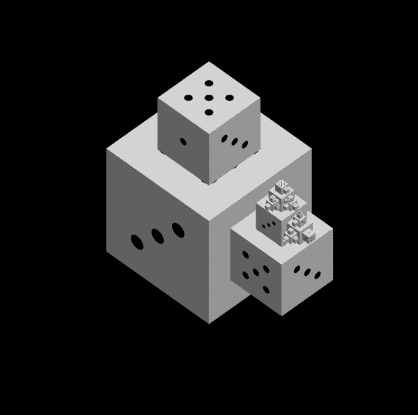
Notice how we only see odd faces on this geometric object? That's because at each roll, we cover up any even faces with another roll until only odd sides are visible. This recursive process repeats on and on, and can create quite interesting results such as above.

Let's try another condition. Say, we'll evaluate if the face is 1. Then we may see an output like this.

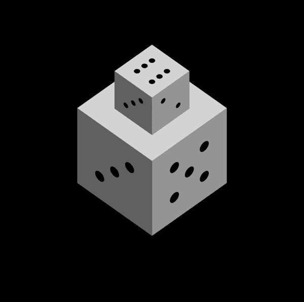
This particular random object contains only two dice. Such a shortly terminated example is more likely to happen with this condition than the previous one. Exactly half of all 24 die corners contain a 1 (count them!). So there's a $1/2$ chance of recursing on the 1 condition. Contrast this with the chances of the even condition — the only corners that do not contain an even face are the $(1,3,5)$, $(3,5,1)$, and $(5,1,3)$ rolls, meaning there is a $21 / 24 = 7/8$ chance of recursing there.

Interesting, now, what would happen if we recurse on every face with 100% probability? We're led to the following picture.

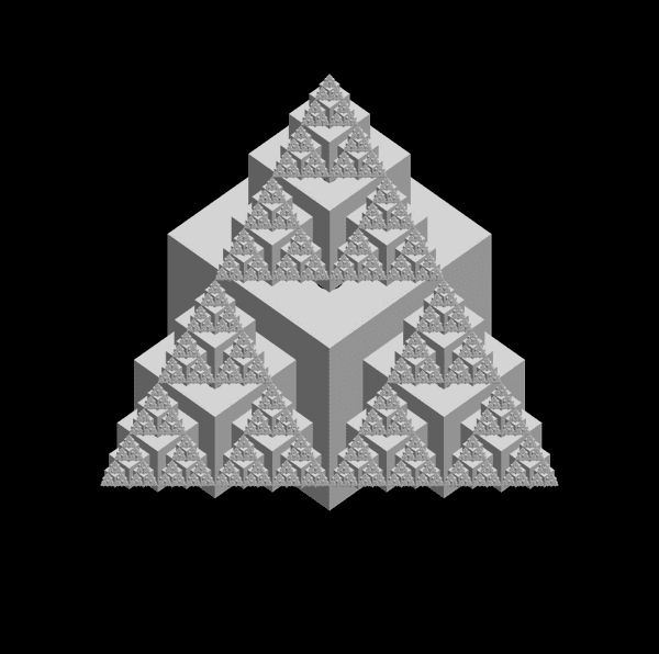
Weird, isn't it? When repeating the process ad infinitum, we see a new geometric feature emerge composed of triangles. To make it clearer, here is a graphic where we show each iteration being generated. I've shifted the positioning of the dice slightly to help illustrate the point and removed the die labels for clarity.

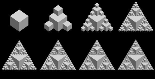
This emerging feature has a name: It's called the Sierpinski gasket (or Sierpinski triangle). It's a well studied fractal, and at first it is quite surprising to see this seemingly unrelated geometric concept appearing in our dice rendering. But, after further consideration, it is not so strange.

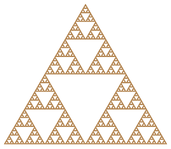
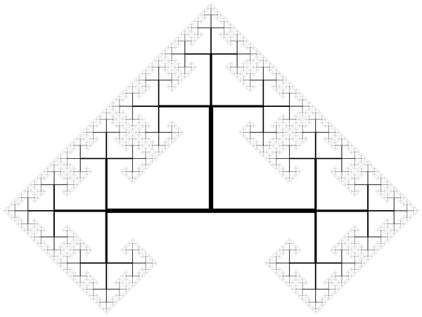
The Sierpinski gasket is not so different from another fractal called the 3-tree. This fractal is produced by starting at a point, drawing 3 branches and recursing on each branch. If anything, the 3 tree sounds almost exactly like the way we are recursing on the dice. The angle at which we branch is not specified, so we can vary that. If we allow 90 degrees between each branch, the fractal looks as follows.

And if we instead render the 3-tree with 120 degrees between each branch:

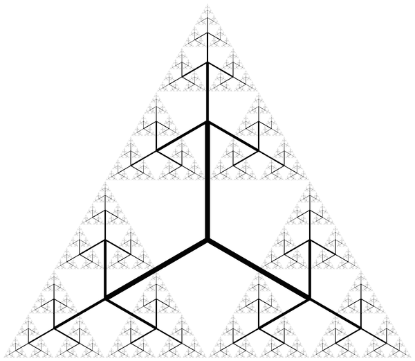
At 120 degrees, the 3-tree suggests again the Sierpinski gasket. But more remarkably, we also see the skeleton of the dice fractal emerge, as well. So clearly, the Sierpinski gasket, the 3-tree and our dice fractal must all be related in some way.

The connection? The 3-tree enumerates a traversal through the complementary space of the gasket. In other words, the 3 tree provides an encoding of the areas not contained in the Sierpinski gasket (the upside down triangles). In this sense, we could consider the 3-tree and the Sierpinski gasket as complementary fractals.

An important concept to fractals is that of fractal dimension. Fractals defy the conventional ideas of 2-dimensional or 3-dimensional Euclidean space and instead occupy spaces which float in between integer dimensions. While there are multiple choices of metrics to compute to the fractal dimension, a common choice is the Hausdorff dimension. Both the Sierpinski gasket and the 3-tree have Hausdorff dimension $\log(3) / \log(2) \approx 1.58$. This says that both fractals are something between 1-dimensional and 2-dimensional objects.

As for our dice fractal, we have happened upon an object embedded in three-dimensional space whose boundary (in limit) contains both the 3-tree and Sierpinski gasket fractals. And, this fact is nicely summarized by the graphics we've explored.

Branching Processes on Fractals

Generalizing on the random walks discussed earlier, we can think of the recursive dice objects as representing a branching process on the 3-tree. Branching processes are an extension of random walks since they allow the current "generation" to reproduce into a larger generation. In rolling a dice corner and acting on each face, we are in essence deciding whether or not to move down a branch of the 3-tree. We end with a subset of the full fractal (or the whole thing if the probability of reproduction is 100%).

A natural question for branching processes is: How likely is it that the branching process will terminate ("ultimate extinction")?

As noted in the Wikipedia article, Wald's equation can be used to answer the question. If the expected number of children $\mu$ of an individual is less than 1, then ultimate extinction happens with probability 1. Conversely, if $\mu > 1$, then ultimate extinction is strictly less than 1.

Let's return to our example of recursing on a die face if it is even. The expected number of recursive die rolls is then $3/2$ (each face is reproduces a single child with probability $1/2$ and by linearity of expectation, the overall expected value for 3 faces is then $3/2$). Hence, we see that ultimate extinction happens with probability less than 1. Which explains why many of the renderings from this rule produce what look like infinitely descending cases.

If we turn our attention to the rule of a reproducing when a face is 1, we instead see $\mu = 1/2$ (each face has a $1/6$ chance of being 1 and then again by linearity of expectation the overall expected value is $3/6$). Here, $\mu < 1$ explains why our renderings always reach ultimate extinction.

In general, if the probability of recursing on a face is $p$, then $\mu = 3p$. Therefore, ultimate extinction is guaranteed for our dice process only when $p < 1/3$.

Conclusion

Altogether, we've used dice to explore a breadth of mathematical fields including some which produce visually interesting graphics like fractals. As I was exploring the different topics of this series, I was often surprised at the connections that were made (e.g., discovering the Sierpinski gasket in the dice rendering). Each new discovery lit a curiosity to investigate what else there was hiding under the surface. From probability, groups, fractals and more, we've seen that even the ordinary die is more than meets the eye. I wonder what other kinds of every day objects could lead to such fascinating results.